|
Statistics for the Behavioral
Sciences |
Lesson 5
Measures of Variability |
Roger N. Morrissette, PhD |
Measures of
Variability tell us the degree to which the scores in a data distribution
vary from the mean score. This can reveal the consistency or similarity of the
scores in a distribution and can indicate just how much the average score
truly represents all the scores in the distribution.
II. The Range
The first type of
variability measure is called the Range. It consists of the full extent
of the scores in a distribution, from the highest score to the lowest score.
The range is severely affected by extreme scores in your data distribution.
Just one of these extreme scores can significantly alter the range. Therefore
the range is not used as a reliable measure of variability. The formula
for the range is shown below:
Range
= high score – low score
III. Average Mean Deviation
The Average Mean Deviation
(AMD) is the average
deviation of each score about the mean of the distribution. To calculate
the average mean deviation you first need to calculate the mean. Next you need
to subtract the mean from all of the raw scores. These scores are now called
the deviation scores or mean deviations and are represented by
little "x." We next sum all the deviation scores and divide by the
total number of scores to get to the average mean deviation. The formula for the
average mean deviation is shown below:
The formula reads:
Average mean deviation equals the sum of all the deviation scores (Xbar or the mean
subtracted from each raw score) divided by the sample size (n). We can abbreviate the
numerator of the equation, the sum of the deviation scores by using the sum of
little x, since little x is the symbol for deviation score.
The major problem with the
Average Mean Deviation is that it always equals zero (as is shown in the
table below). This makes it impossible to compare the variability of one
distribution with another. Therefore the average mean
deviation is not used as a reliable measure of variability.
|
X |
x
or (X - Xbar) |
x
or (X - Xbar) |
| 1 |
1 - 3 |
-2 |
| 2 |
2 - 3 |
-1 |
| 3 |
3 - 3 |
0 |
| 4 |
4 - 3 |
1 |
| 5 |
5 - 3 |
2 |
| Σ X = 15 |
n = 5 |
Σ x = 0 |
|
Xbar
= 15 / 5 |
|
AMD = 0 / 5 |
|
Xbar = 3 |
|
AMD =
0 |
IV. The Relationship
Between Population/Sample and Variance/Standard Deviation (Video
Lesson 5 IV) (YouTube
version)
As you might remember from
Lesson 1, Populations are big and Samples are
small. Samples are taken from an overall Population. Statistics are calculated
on Samples not Populations because Populations are too big and the data is
virtually impossible to collect. The results from a "good" Sample can be
inferred to the overall Population. That said we still have statistics for
Populations. The "Variance" gets around the problem of average
mean deviation by squaring the deviation scores. The "Standard Deviation"
is simply the square root of the Variance and gives us a more realistic value of
deviation about the means. The calculation of both Variance and Standard
Deviation are discussed in section V and VI respectively. Below are the
Population and Sample formulas for both Variance and
Standard Deviation. Please make a note of the differences between the
two but know that you will ONLY
be using the Sample formulas for the homework and examinations.
| Variance |
Standard Deviation |
Population Variance (Non-Computational
formula) |
Population Standard Deviation
(Non-Computational formula) |
Sample Variance (Non-Computational formula) |
Sample Standard Deviation (Non-Computational
formula) |
Sample Variance (Computational formula) |
Sample Standard Deviation (Computational
formula) |
Sample Variance (Grouped Frequency formula) |
Sample Standard Deviation (Grouped
Frequency formula) |
V. Variance
One way to get
around the problem of the average mean deviation always equaling to zero is to
simply square the
deviation scores. By doing this we are on our way to calculate the Variance
or the mean of the squared differences. The first step is to calculate the mean
as we did in solving for the average mean deviation. We must then again subtract
the mean from all of the raw scores to get the deviation scores.
Now we square all of the deviation scores, sum them, and divide by the total
number of scores minus 1. Just as we did with measures of central
tendency, we can calculate the variance for raw data and grouped
frequency data. We can also calculate the variance for both a population
and a sample and there are two different formulas you can use, the
non-computational formula and the computational formula.
A. Raw Data
Collection:
The non-computational
formula for the variance of a population using raw data is:
The formula reads: sigma
squared (variance of a population) equals the sum of all the squared deviation
scores of the population (raw scores minus mu or the mean of the population)
divided by capital N or the number of scores in the population.
The non-computational
formula for the variance of a sample using raw data is: (Video
Lesson 5 VA1) (YouTube
version) (Raw Data Standard Deviation/Variance Calculation - YouTube
version) (mp4 version)
The formula reads: capital
S squared (variance of a sample) equals the sum of all the squared deviation
scores of the sample (raw scores minus x bar or the mean of the sample) divided
by lower case n or the number of scores in the sample minus 1.
To solve the
non-computational formula for the variance of a sample using raw
data we first take our raw scores, put them in a table, calculate the mean,
calculate the deviation scores, square the deviation scores and then sum the
squared deviation scores:
Raw score data:
2 4 5 1 3
|
X |
x
or (X - Xbar) |
x
or (X - Xbar) |
x2 or (X - Xbar)2 |
| 2 |
2 - 3 |
-1 |
1 |
| 4 |
4 - 3 |
1 |
1 |
| 5 |
5 - 3 |
2 |
4 |
| 1 |
1 - 3 |
-2 |
4 |
| 3 |
3 - 3 |
0 |
0 |
| Σ X = 15 |
|
|
Σ
x2 = 10 |
| n = 5 |
Xbar
= 15 / 5 |
|
or |
| |
Xbar = 3 |
|
Σ (X
- Xbar)2
= 10 |
Now we can solve the
non-computational formula for the variance of a sample using raw
data:
S2
= Σ (X - Xbar)2/
n - 1
S2
= 10 / 5 - 1
S2
= 10 / 4
S2
= 2.5
The variance for
the data set above is 2.5.
The computational
formula for the variance of a sample using raw data is: (Video
Lesson 5 VA2) (YouTube
version) (Raw Data Standard Deviation/Variance Calculation - YouTube
version) (mp4 version)
The formula reads: capital
S squared (variance of a sample) equals the sum of all the raw scores squared
minus the sum of all the raw scores then squared and divided by the sample size.
This entire numerator is then divided by the sample size minus 1.
To solve the
computational formula for the variance of a sample using raw data
we first take our raw scores, put them in a table, square them, and sum the
squared values:
Raw score data:
2 4 5 1 3
|
X |
X2 |
| 2 |
4 |
| 4 |
16 |
| 5 |
25 |
| 1 |
1 |
| 3 |
9 |
| Σ X =
15 |
Σ X2
= 55 |
| n = 5 |
|
Now we can solve the
computational formula for the variance of a sample using raw data:
S2
= (Σ X2
- (Σ X)2
/ n) / n - 1
S2
= (55 - (15)2 / 5)
/ 5 - 1
S2
= (55 - 225/ 5) / 4
S2
= (55 - 45) / 4
S2
= 10 / 4
S2
= 2.5
The variance for
the data set above is 2.5. Notice how
both the non-computational formula and computational formula came up with the
exact same answer. You can use which ever one you are more comfortable with to
solve the variance problems on the exam.
B. Grouped
Frequency Data: (Video
Lesson 5 VB) (YouTube
version) (Grouped Frequency Standard Deviation/Variance
Calculation - YouTube version) (mp4 version)
When you do not have raw data but instead have only Grouped Frequency Data,
as is shown in the table below, the calculation of the variance is a bit different.
| Apparent Limits |
Frequency |
| 81-90 |
5 |
| 71-80 |
3 |
| 61-70 |
12 |
| 51-60 |
16 |
| 41-50 |
33 |
| 31-40 |
21 |
| 21-30 |
15 |
| 11-20 |
7 |
| Sum |
112 |
The formula for the
variance of a sample using grouped frequency data is:
The formula reads: capital
S squared (variance of a sample) equals the sum of all the frequencies
multiplied by the square of their deviation scores and then the entire numerator
is divided by the sample size minus 1. CAUTION:
remember that little x equals (MIDPOINT - Xbar)
To solve the formula we
first make a column for midpoints and frequency times midpoints,
then calculate the mean.
| Apparent Limits |
Frequency |
Midpoints |
Frequency x Midpoints |
| 81-90 |
5 |
85.5 |
427.5 |
| 71-80 |
3 |
75.5 |
226.5 |
| 61-70 |
12 |
65.5 |
786 |
| 51-60 |
16 |
55.5 |
888 |
| 41-50 |
33 |
45.5 |
1501.5 |
| 31-40 |
21 |
35.5 |
745.5 |
| 21-30 |
15 |
25.5 |
382.5 |
| 11-20 |
7 |
15.5 |
108.5 |
| Sum |
112 |
|
5066 |
Xbar =
Σ (Frequency x Midpoint) /
n
Xbar = 5066
/ 112
Xbar
= 45.23
Using the mean we can now
generate a deviation score column, a squared deviation score
column, a frequency times squared deviation score column and the sums of
the columns:
| Apparent Limits |
Frequency |
Midpoints |
Frequency x Midpoints |
x or
(Midpoint -Xbar) |
x2 or
(Midpoint -Xbar)2 |
Frequency x (Midpoint -Xbar)2 |
| 81-90 |
5 |
85.5 |
427.5 |
40.27 |
1621.673 |
8108.365 |
| 71-80 |
3 |
75.5 |
226.5 |
30.27 |
916.273 |
2748.819 |
| 61-70 |
12 |
65.5 |
786 |
20.27 |
410.873 |
4930.475 |
| 51-60 |
16 |
55.5 |
888 |
10.27 |
105.473 |
1687.566 |
| 41-50 |
33 |
45.5 |
1501.5 |
0.27 |
0.073 |
2.406 |
| 31-40 |
21 |
35.5 |
745.5 |
-9.73 |
94.673 |
1988.131 |
| 21-30 |
15 |
25.5 |
382.5 |
-19.73 |
389.273 |
5839.094 |
| 11-20 |
7 |
15.5 |
108.5 |
-29.73 |
883.873 |
6187.11 |
| Sum |
112 |
|
|
|
|
31491.96 |
| |
|
|
Xbar
=
45.23 |
|
|
|
S2
=
Σ (F ·
x2)
/ n - 1
S2
= 31491.96 /
112 - 1
S2
= 31491.96 /
111
S2
= 283.711
The
variance for the data set above is 283.711.
The Standard Deviation
is simply the square root of the variance. It
represents an average measure of the amount each score deviates from the mean.
The standard deviation is in the same units as the original raw scores so is an
ideal measure of variability. Just as we did with measures of central
tendency and variance, we can calculate the standard deviation for raw data
and grouped frequency data. We can also calculate the standard deviation
for both a population and a sample and there are two different
formulas you can use, the non-computational formula and the
computational formula. All of these formulas are calculated in the
exact manner as solving for variance except that once you have found the
variance you simply take the square root of that value to determine the standard
deviation.
The non-computational
formula for the standard deviation of a population using raw data
is:
The formula reads: sigma
(standard deviation of a population) equals the square root of the sum of all
the squared deviation scores of the population (raw scores minus mu or the mean
of the population) divided by capital N or the number of scores in the
population.
The non-computational
formula for the standard deviation of a sample using raw data
is:
The formula reads: capital
S (standard deviation of a sample) equals the square root of the sum of all the
squared deviation scores of the sample (raw scores minus x bar or the mean of
the sample) divided by lower case n or the number of scores in the sample minus
1.
The computational
formula for the standard deviation of a sample using raw data is:
The formula reads: capital
S (standard deviation of a sample) equals the square root of the sum of all the
raw scores squared minus the sum of all the raw scores then squared and divided
by the sample size. This entire numerator is then divided by the sample size
minus 1.
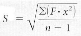
The formula for the
standard deviation of a sample using grouped frequency data is:
The formula reads: capital
S (standard deviation of a sample) equals the square root of the sum of all the
frequencies multiplied by the square of their deviation scores and then the
entire numerator is divided by the sample size minus 1.
CAUTION: remember that little x
equals (MIDPOINT - Xbar)
Additional Videos on the Concepts that might help:
Range, Variance,
Standard Deviation
How to Calculate Standard
Deviation and Variance
What is Variance in
Statistics?
Finding the Standard
Deviation of a Data Set
Standard Deviation