|
Statistics for the Behavioral Sciences |
Lesson 7 Correlation |
Roger N. Morrissette, PhD |
A correlation is a statistical test that demonstrates the relationship between two variables. Even though you may be able to show a significant relationship between two variables, a correlation does not show a causal relationship between the two variables. For example, although depression and self-esteem are two variables that are significantly correlated to each other we can not say that low self-esteem causes depression. Likewise, we can not say that depression causes low self-esteem. The two variables may be significantly correlated but no causal relationship is assumed. Correlations are best represented graphically by a scatterplot and best calculated by using the Pearson Product Moment Correlation formula.
Let's test this hypothesis that depression scores are negatively correlated to self-esteem scores. We design our surveys and sample 8 subjects. Their data is presented below. Data for a correlation are always presented in two columns like the data set shown below. Depression scores are our X data and Self-Esteem Scores are our Y data:
Depression (X)
Self-Esteem (Y)
10
104
12
100
19
98
4
150
25
75
15
105
21
82
7
133
II. Scatterplots (Video Lesson 7 II) (YouTube version)
A scatterplot is a graphical representation of the two sets of data you are comparing. The X-axis plots your first or "X" data, and the Y-axis plots your second or "Y" set of data. The scatterplot can tell you two important things about the relationship between your two variables. First it can show you if you have a weak or strong relationship between your variables. Secondly, it can tell you if your variables are negatively or positively related.
A. Scatterplots can show the strength of the relationship between two variables
1. Weak relationships will have a wide scattering of the plots
2. Strong relationships will have a minimal scattering of the plots
both factors vary in the same direction
as one factor increases, the other increases
both factors vary in opposite directions
as one factor increases, the other decreases
the two factors show no relationship to one another
The correlation coefficient is a statistic that calculates the actual relationship between two variables. It has a range between -1.00 and +1.00. You can not get a correlation of 1.5. A value of -1.00 would be a perfect (very strong) negative correlation, a value of +1.00 would be a perfect (very strong) positive correlation, and a value of 0.00 would be a (very weak) zero or neutral correlation. To calculate the correlation coefficient we use the Pearson Product Moment Correlation (r):
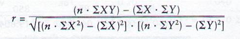
The formula reads: r equals. In the numerator: n or number of pairs multiplied by the sum of X and Y then subtract the sum of X times the sum of Y. In the denominator: Take the square root of the final sum of n times the sum of X squared minus the sum of X then squared, then multiply that value by n times the sum of Y squared, then minus the sum of Y then squared.
|
Depression (X) |
Self-Esteem (Y) |
|
10 |
104 |
|
12 |
100 |
|
19 |
98 |
|
4 |
150 |
|
25 |
75 |
|
15 |
105 |
|
21 |
82 |
|
7 |
133 |
To calculate the correlation coefficient (r) for the data above we first need to expand the columns just as we did when we calculated standard deviation. If you look at the formula above you will see that we need an X squared column, a Y squared column and an X times Y column. This first step is show below:
|
X |
Y |
X2 | Y2 | XY |
|
10 |
104 |
100 | 10816 | 1040 |
|
12 |
100 |
144 | 10000 | 1200 |
|
19 |
98 |
361 | 9604 | 1862 |
|
4 |
150 |
16 | 22500 | 600 |
|
25 |
75 |
625 | 5625 | 1875 |
|
15 |
105 |
225 | 11025 | 1575 |
|
21 |
82 |
441 | 6724 | 1722 |
|
7 |
133 |
49 | 17689 | 931 |
The next step is to calculate the sums of our columns:
|
X |
Y |
X2 | Y2 | XY |
|
10 |
104 |
100 | 10816 | 1040 |
|
12 |
100 |
144 | 10000 | 1200 |
|
19 |
98 |
361 | 9604 | 1862 |
|
4 |
150 |
16 | 22500 | 600 |
|
25 |
75 |
625 | 5625 | 1875 |
|
15 |
105 |
225 | 11025 | 1575 |
|
21 |
82 |
441 | 6724 | 1722 |
|
7 |
133 |
49 | 17689 | 931 |
| 113 | 847 | 1961 | 93983 | 10805 |
| n = 8 |
|
Now we have all the information we need to solve our equation:
r = (8 x 10805) - (113 x 847) / square root [(8 x 1961) - (113)2] x [(8 x 93983) - (847)2]
r = (86440) - (95711) / square root [(15688) - (12769)] x [(751864) - (717409)]
r = - 9271 / square root [(2919) x (34455)]
r = - 9271 / square root (100574145)
r = - 9271 / 10028.666
r = - 0.9244
Our correlational coefficient is negative and very close to 1.00 which tells us that we have a strong negative relationship between our two variables. If we look at the scatterplot of our data we can see that the scatterplot is in aligned with our correlational coefficient.
Now that we have calculated our correlation coefficient we need determine how significant it is. There are two ways to determine the significance of a correlation: the first is to calculate the Coefficient of Determination and the second is to use the R Table.
The coefficient of determination determines how much of the variance of one factor can be explained by the variability of a factor with which it is correlated. To calculate the coefficient of determination we simply square the r value.
Coefficient of Determination = r2
For our r of - 0.9244, the coefficient of determination would be r2 = 0.8545. This means that 85% of the variance of our depression scores can be explained by the variance of our self-esteem scores. This is a pretty high value and suggests a very strong relationship between the two variables. Although the coefficient of determination is a good predictor of the strength of the relationship between two variables, it does not predict significance. We will need to use the R Table to confirm if our correlation is statistically significant.
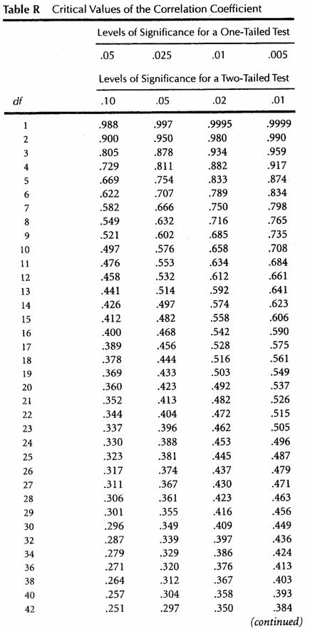
The R Table is located in its entirety in Appendix A in the back of the text book. A shortened version is also available at the bottom of this lecture. It starts on page 435 and gives the critical R values based on degrees of freedom of your sample, the level of significance of the statistical test, and whether your hypothesis is one- or two-tailed. These three factors plus the critical R values are represented in the R Table and will be explained one at a time.
1. Degrees of Freedom.
The term degrees of freedom refers to the number of scores within a data set that are free to vary. In any sample with a fixed mean, the sum of the deviation scores is equal to zero. If your sample has an n equal to 10. The first 9 scores are free to vary but the 10th score must be a specific value that makes the entire distribution equal to zero. Therefore in a single sample the degrees of freedom would be equal to n - 1. The degrees of freedom for a correlation is slightly different because n equals number of pairs not simply sample size. Therefore, the degrees of freedom for a correlation in n - 2. So to calculate the degrees of freedom you simply take the number of pairs and subtract two. For our data set of depression and self-esteem scores the degrees of freedom are calculated the following way:
df = n -2
df = 8 - 2
df = 6
The R Table shows the degrees of freedom values in the far left column as shown below:
| Levels of Significance for a One-Tailed Test |
| .05 | .025 | .01 | .005 |
| Levels of Significance for a Two-Tailed Test |
| df | .10 | .05 | .02 | .01 |
| 1 | .988 | .997 | .9995 | .9999 |
| 2 | .900 | .950 | .980 | .990 |
| 3 | .805 | .878 | .934 | .959 |
| 4 | .729 | .811 | .882 | .917 |
| 5 | .669 | .754 | .833 | .874 |
| 6 | .622 | .707 | .789 | .834 |
| 7 | .582 | .666 | .750 | .798 |
| 8 | .549 | .632 | .716 | .765 |
| 9 | .521 | .602 | .685 | .735 |
| 10 | .497 | .576 | .658 | .708 |
The table continues
2. One- or Two-tailed hypotheses.
The number of tails of a hypothesis predict the direction of the hypothesis. This concept will be discussed in greater detail in chapter 11. For now, you should know that if a correlation hypothesis is simply predicting an effect without predicting either a negative or positive direction of that effect, it is considered a Two-Tailed hypothesis. If the hypothesis is predicting either a negative or positive direction then it is a One-Tailed hypothesis. Since our hypothesis as stated predicts a negative correlation it is a One-Tailed Test. The two levels of hypothesis tests are highlighted below:
| Levels of Significance for a One-Tailed Test |
| .05 | .025 | .01 | .005 |
| Levels of Significance for a Two-Tailed Test |
| df | .10 | .05 | .02 | .01 |
| 1 | .988 | .997 | .9995 | .9999 |
| 2 | .900 | .950 | .980 | .990 |
| 3 | .805 | .878 | .934 | .959 |
| 4 | .729 | .811 | .882 | .917 |
| 5 | .669 | .754 | .833 | .874 |
| 6 | .622 | .707 | .789 | .834 |
| 7 | .582 | .666 | .750 | .798 |
| 8 | .549 | .632 | .716 | .765 |
| 9 | .521 | .602 | .685 | .735 |
| 10 | .497 | .576 | .658 | .708 |
3. Levels of Significance.
The levels of significance or "p values" will also be discussed in greater detail in chapters 11, 12, and 13. For now you should simply know that a level of significance at .05 is equivalent to p = .05 which means that there is a 95% probability of statistical significance (1.00 - 0.05 = 0.95 or 95%) between your two variables. The .05 value is considered standard in science. Levels of significance that are smaller show greater significance and values that are larger show less significance. This value must be given to you in the problem. For our example let's use a p = .05. The table below shows the highlighted levels of significance:
| Levels of Significance for a One-Tailed Test |
| .05 | .025 | .01 | .005 |
| Levels of Significance for a Two-Tailed Test |
| df | .10 | .05 | .02 | .01 |
| 1 | .988 | .997 | .9995 | .9999 |
| 2 | .900 | .950 | .980 | .990 |
| 3 | .805 | .878 | .934 | .959 |
| 4 | .729 | .811 | .882 | .917 |
| 5 | .669 | .754 | .833 | .874 |
| 6 | .622 | .707 | .789 | .834 |
| 7 | .582 | .666 | .750 | .798 |
| 8 | .549 | .632 | .716 | .765 |
| 9 | .521 | .602 | .685 | .735 |
| 10 | .497 | .576 | .658 | .708 |
4. Critical R Values.
Critical values are threshold values for significance. Your calculated r value must exceed the critical r value in the R Table to be considered significant. The table below shows the highlighted critical r values:
| Levels of Significance for a One-Tailed Test |
| .05 | .025 | .01 | .005 |
| Levels of Significance for a Two-Tailed Test |
| df | .10 | .05 | .02 | .01 |
| 1 | .988 | .997 | .9995 | .9999 |
| 2 | .900 | .950 | .980 | .990 |
| 3 | .805 | .878 | .934 | .959 |
| 4 | .729 | .811 | .882 | .917 |
| 5 | .669 | .754 | .833 | .874 |
| 6 | .622 | .707 | .789 | .834 |
| 7 | .582 | .666 | .750 | .798 |
| 8 | .549 | .632 | .716 | .765 |
| 9 | .521 | .602 | .685 | .735 |
| 10 | .497 | .576 | .658 | .708 |
Now let's put it all together. The table below shows the criteria of our example to determine if our calculated r value of is significant:
| Levels of Significance for a One-Tailed Test |
| .05 | .025 | .01 | .005 |
| Levels of Significance for a Two-Tailed Test |
| df | .10 | .05 | .02 | .01 |
| 1 | .988 | .997 | .9995 | .9999 |
| 2 | .900 | .950 | .980 | .990 |
| 3 | .805 | .878 | .934 | .959 |
| 4 | .729 | .811 | .882 | .917 |
| 5 | .669 | .754 | .833 | .874 |
| 6 | .622 | .707 | .789 | .834 |
| 7 | .582 | .666 | .750 | .798 |
| 8 | .549 | .632 | .716 | .765 |
| 9 | .521 | .602 | .685 | .735 |
| 10 | .497 | .576 | .658 | .708 |
According to Table R, For a One-Tailed test at p = .05 with 6 degrees of freedom the critical value we must exceed to consider our calculated r value to be significant is .622.
Since our calculated r = -0.9244
We conclude that our correlation is significant.
*Note that the final cumulative percent score should equal 100%
| Additional Links about the Concepts that might help: |
|
How to Calculate the Correlation Coefficient |